AWS Cost Allocation and FinOps Architecture Deep Dive
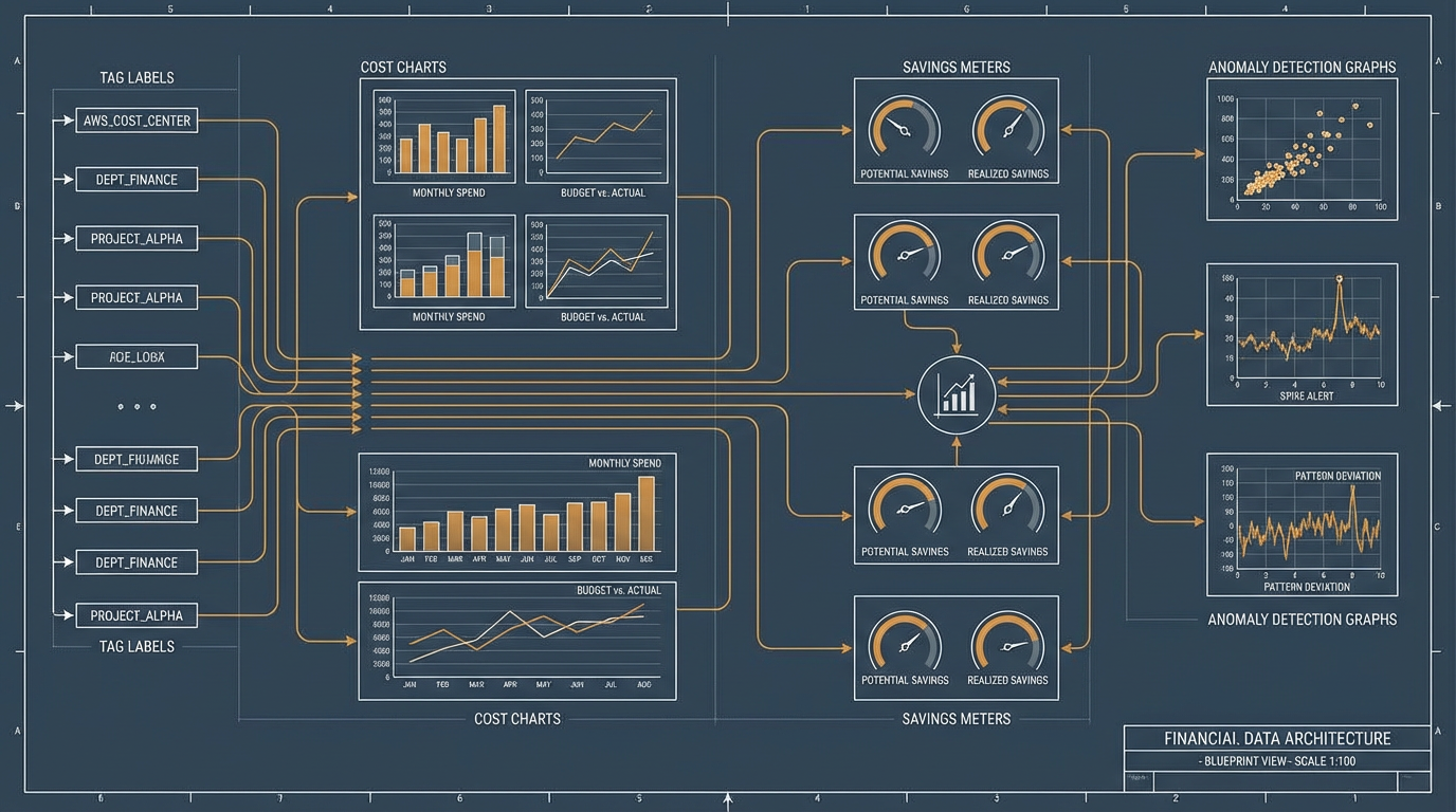
I have managed AWS spend across organizations ranging from $50,000 to $8 million per month. The single biggest difference between organizations that control their cloud costs and those that hemorrhage money is not tooling or dashboards. It is architecture. Specifically, whether cost allocation was designed into the platform from day one or bolted on after the CFO started asking uncomfortable questions. This article covers the architecture I build for every engagement: tagging strategies that survive real-world entropy, CUR analysis pipelines that produce actionable data, anomaly detection that catches problems before they become invoices, and commitment optimization that maximizes discount capture without over-committing.
The Cost Allocation Foundation: Tagging Architecture
Tags are the atomic unit of cost allocation. Every dollar AWS charges can be attributed to a business function, team, environment, or project only if the resource that generated the charge carries the right tags. Get tagging wrong and everything downstream (reports, anomaly detection, chargeback, optimization) produces garbage.
Tag Taxonomy Design
I use a four-tier taxonomy that balances granularity with compliance burden:
| Tier | Tag Key | Example Values | Purpose |
|---|---|---|---|
| Financial | CostCenter, BillingCode |
CC-4200, PROJ-AVIAN |
Chargeback to P&L |
| Organizational | Team, Owner |
platform-eng, csieg@company.com |
Accountability |
| Operational | Environment, Service |
production, auth-service |
Filtering and analysis |
| Lifecycle | CreatedBy, ExpiresOn |
terraform, 2026-06-01 |
Cleanup and governance |
Financial tags drive chargeback. Organizational tags drive accountability. Operational tags drive analysis. Lifecycle tags drive hygiene. Every resource needs at least one tag from each tier.
User-Defined vs. AWS-Generated Tags
AWS provides two categories of cost allocation tags, and understanding the distinction matters for architecture:
AWS-generated tags start with the aws: prefix and are created automatically. The most useful is aws:createdBy, which tracks who or what created a resource. These tags do not count against tag quotas and are only available in the Billing Console and CUR. You cannot use them in IAM policies or resource-level operations.
User-defined tags are what you create and manage. They appear in billing reports only after you explicitly activate them in the Billing Console. The activation lag is up to 24 hours, and tags are not retroactive. If you tag a resource on March 15, cost data before March 15 will not carry that tag. This has a critical architectural implication: tag compliance must be enforced at resource creation time, not after the fact.
Tag Limits
| Constraint | Limit |
|---|---|
| User-defined tags per resource | 50 |
| Tag key maximum length | 128 characters (UTF-8) |
| Tag value maximum length | 256 characters (UTF-8) |
| Active cost allocation tag keys per account | 500 |
| AWS-generated tags | Do not count against limits |
| Billing appearance lag | Up to 24 hours |
| Retroactive application | Not supported |
Fifty tags per resource sounds generous until you realize that Terraform modules, Kubernetes controllers, and CI/CD pipelines all add their own tags. I have seen production resources hit the limit. Design your taxonomy to use no more than 15-20 tag keys, leaving headroom for tooling.
Tag Propagation: The Hidden Problem
Not all AWS services propagate tags consistently. This is the single biggest source of unallocated cost in most organizations.
| Service | Propagation Behavior |
|---|---|
| EC2 Auto Scaling | Tags copied to launched instances automatically |
| RDS | DB instance tags propagated to snapshots |
| ECS | Tags propagated to tasks via PropagateTags parameter (must be enabled) |
| EMR | Cluster tags propagated to launched instances by default |
| ElastiCache | Replication group tags propagate to clusters |
| EKS (Fargate) | Profile tags do NOT propagate to Pods |
| Lambda | Function tags do NOT propagate to CloudWatch Logs log groups |
| S3 | Bucket tags do NOT propagate to objects |
| CloudFormation | Stack tags propagated to created resources (most services) |
The EKS gap is particularly painful. If you run Kubernetes workloads on Fargate, the Fargate profile tags do not flow to the underlying compute. You need Kubecost or a CloudTrail-based automation pipeline to attribute costs to namespaces and workloads.
Enforcing Tag Compliance
Tag compliance degrades exponentially without enforcement. After 90 days, a voluntary tagging policy typically covers 40-60% of resources. After a year, it is below 30%. I enforce at three layers:
Layer 1: Service Control Policies (SCPs) block resource creation without required tags. This is the hardest gate and the most effective. An SCP that denies ec2:RunInstances without an Environment tag means no untagged EC2 instances can exist.
Layer 2: AWS Tag Policies enforce tag key naming conventions and allowed values at the organization level. They prevent environment vs. Environment vs. env drift and restrict values to a defined set (production, staging, development).
Layer 3: AWS Config Rules monitor compliance continuously and can trigger auto-remediation via Lambda. The required-tags managed rule checks for tag presence; custom rules can validate tag values against a canonical list.
The three layers work together: SCPs prevent creation of non-compliant resources, Tag Policies prevent structural drift, and Config Rules catch anything that slips through (imported resources, API-created resources that bypass SCPs).
Cost and Usage Reports: The Data Pipeline
The Cost and Usage Report (CUR) is the foundation of every serious FinOps program. It is the most granular billing data AWS provides: every line item, every resource, every hour, every tag. Everything else (Cost Explorer, Budgets, Anomaly Detection) is a view on top of CUR data.
CUR 2.0 vs. Legacy CUR
AWS replaced the legacy CUR format with CUR 2.0 through the Data Exports service. The differences matter for pipeline architecture:
| Aspect | Legacy CUR | CUR 2.0 |
|---|---|---|
| Schema stability | Variable columns monthly (100-500+) | Fixed schema (~125 columns) |
| Tag columns | Individual column per tag key | Nested JSON in resource_tags |
| Cost Category columns | Individual column per category | Nested JSON in cost_categories |
| Discount columns | Individual per discount type | Nested in discount group |
| Format | CSV or Parquet | Parquet (default, 30-90% smaller) |
| Column selection | All or nothing | Select specific columns |
| Business unit filtering | Not supported | Filter by account or tag |
CUR 2.0 is a significant improvement. The fixed schema means your Athena queries do not break when AWS adds a new service or you create a new tag. The nested JSON approach for tags and categories reduces column count dramatically. The column selection feature means you can create multiple exports tailored to different teams, each containing only the data they need.
Key CUR Columns
The CUR schema is large, but these columns drive 90% of analysis:
| Column Group | Key Columns | Purpose |
|---|---|---|
| Bill | bill_payer_account_id, bill_billing_period_start_date |
Identify which org and period |
| Line Item | line_item_type, line_item_usage_account_id, line_item_product_code |
What was used, by whom |
| Usage | line_item_usage_amount, line_item_usage_start_date |
How much, when |
| Cost | cost_amortized_cost, cost_unblended_cost, cost_net_amortized_cost |
How much it cost (three views) |
| Pricing | pricing_term, pricing_public_on_demand_rate |
On-Demand vs. Reserved vs. Spot |
| Reservation | reservation_reservation_arn, reservation_amortized_upfront_fee |
RI attribution |
| Savings Plan | savings_plan_savings_plan_arn, savings_plan_savings_plan_rate |
SP attribution |
| Resource | line_item_resource_id, resource_tags |
Which resource, with what tags |
Understanding Cost Types
This is where most FinOps programs get confused. AWS provides four cost views in CUR, and choosing the wrong one produces misleading reports.
Unblended cost is what you were actually charged on the day the usage occurred. If you bought a 1-year All Upfront RI for $12,000, the unblended cost shows $12,000 on the purchase date and $0 for the next 364 days. This matches your invoice but is useless for trend analysis.
Amortized cost spreads commitment fees evenly across the term. That $12,000 RI shows as ~$32.88/day for 365 days. This is the right view for budgeting, forecasting, and team-level cost allocation. It answers "what does this workload actually cost per month?"
Net unblended cost is unblended minus discounts (EDPs, private pricing). Use this for invoice reconciliation.
Net amortized cost is amortized minus discounts. This is the truest view of actual economic cost and the one I use for all chargeback models.
| Cost Type | Best For | Avoid For |
|---|---|---|
| Unblended | Invoice reconciliation | Trend analysis, budgeting |
| Amortized | Budgeting, forecasting, team allocation | Invoice matching |
| Net unblended | Discount impact analysis | Day-to-day reporting |
| Net amortized | Chargeback, true economic cost | Comparing to invoice |
Athena Pipeline Architecture
The standard CUR analysis pipeline uses S3, Glue, and Athena:
- CUR delivery to S3: AWS delivers updated data up to 3 times daily, partitioned by year/month.
- Glue Crawler: A CloudFormation-deployed crawler detects new CUR files and updates the Glue Data Catalog schema.
- Partition projection: Instead of physical Glue catalog entries, Athena dynamically calculates partition values. This eliminates the crawler bottleneck for large datasets.
- Athena queries: Analysts and dashboards query the data using standard SQL.
For organizations with 50+ accounts and 12+ months of history, CUR data can reach hundreds of gigabytes. Optimization matters:
| Optimization | Impact |
|---|---|
| Parquet format (vs. CSV) | 30-90% reduction in query cost and time |
| Partition by year/month | Eliminates scanning irrelevant months |
| Column selection in CUR 2.0 export | Reduces export size by 40-70% |
| WHERE clause on partition columns | Mandatory for cost control |
| Athena Workgroups with query cost limits | Prevents runaway queries |
| S3 Lifecycle rules (Glacier after 24 months) | Reduces storage cost for historical data |
Anomaly Detection Architecture
AWS Cost Anomaly Detection uses machine learning to identify unusual spending patterns. It learns from your historical data and adjusts for trends, seasonality, and growth. The architecture is straightforward, but the configuration choices determine whether it produces signal or noise.
Monitor Design
Anomaly Detection supports four monitor dimensions. I deploy all four in a layered configuration:
| Monitor Type | Scope | Catches |
|---|---|---|
| AWS Services | All services across account | New service adoption, service-level spikes |
| Linked Accounts | Per-account spend | Account-level budget blowouts |
| Cost Allocation Tags | Per-tag-value spend | Team or project overspend |
| Cost Categories | Per-category spend | Business unit anomalies |
AWS-managed monitors automatically track the top 5,000 values within a dimension. For most organizations, this covers everything without configuration. Customer-managed monitors let you select up to 10 specific values for aggregate monitoring when you need tighter control.
Threshold Configuration
The default thresholds (40% above expected AND $100 minimum impact) are reasonable for most workloads. I adjust based on account profile:
| Account Type | Percentage Threshold | Absolute Threshold | Rationale |
|---|---|---|---|
| Production (high spend) | 20% | $500 | Small percentage = large dollars |
| Development | 50% | $50 | Expect more variance |
| Sandbox | 100% | $25 | Catch runaway experiments early |
| Shared services | 15% | $1,000 | Tight control on shared infrastructure |
Alert Pipeline
The integration path is: Anomaly Detection -> SNS Topic -> AWS Chatbot -> Slack channel. I add a Lambda function between SNS and Chatbot that enriches the alert with:
- The specific resources driving the anomaly (from CUR data)
- The tag values on those resources (team, owner, environment)
- A direct link to the Cost Explorer filtered view
- Historical context (is this a known pattern or genuinely new?)
The enrichment step transforms a generic "spending anomaly detected" alert into an actionable "auth-service in production spiked 340% due to 47 new c5.2xlarge instances launched by the platform-eng team's Auto Scaling group at 2:15 AM." The second version gets investigated. The first gets ignored.
Custom Anomaly Detection for Granular Control
For workloads where the built-in service is too coarse, I build custom detection using CloudWatch metrics and Lambda:
- CloudWatch custom metrics: Publish hourly spend per service/account/tag from CUR data.
- CloudWatch Anomaly Detector: Apply anomaly detection bands to each metric.
- CloudWatch Alarms: Trigger when spend exceeds the anomaly band.
- Lambda: Enrich and route to Slack/PagerDuty.
This approach gives you sub-hourly detection granularity and full control over the detection algorithm. The trade-off is operational overhead: you are running and maintaining the pipeline yourself.
Commitment Optimization: RIs and Savings Plans
Reserved Instances and Savings Plans are the largest single lever for cost reduction in most AWS organizations. A well-optimized commitment portfolio saves 30-50% on compute spend. A poorly optimized one wastes money on unused reservations while leaving On-Demand spend uncovered.
The Commitment Landscape
| Commitment Type | Max Discount | Flexibility | Best For |
|---|---|---|---|
| Standard RI (3yr, All Upfront) | 72% | Lowest (locked to instance type) | Stable, predictable baselines |
| Convertible RI (3yr, All Upfront) | 66% | Medium (can change family/size) | Growing workloads in known families |
| EC2 Instance Savings Plan (3yr, All Upfront) | 72% | High (any size in family, any AZ) | Stable EC2 within a family |
| Compute Savings Plan (3yr, All Upfront) | 66% | Highest (EC2, Lambda, Fargate) | Mixed compute, multi-service |
| Compute Savings Plan (1yr, No Upfront) | 28% | Highest | Conservative first commitment |
| SageMaker Savings Plan | Up to 64% | SageMaker usage types only | ML training/inference |
The Commitment Stacking Strategy
I build commitment portfolios in layers, from most flexible to most locked:
Layer 1: Compute Savings Plans cover the baseline that you know will exist regardless of architectural changes. Start with 60-70% of your minimum sustained compute spend. These apply to EC2, Lambda, and Fargate, so even if you migrate from EC2 to containers, the commitment still saves money.
Layer 2: EC2 Instance Savings Plans cover the stable portion of specific instance families. If you run m5.xlarge instances 24/7 in production and have no plans to change families, an Instance SP gives you 72% discount versus 66% from Compute SP. The extra 6% adds up at scale.
Layer 3: Convertible RIs cover workloads where you need the ability to change instance types but want deeper discounts than Savings Plans provide for specific configurations.
Layer 4: Standard RIs are only for workloads that will not change for 3 years. Database instances (RDS, ElastiCache) on fixed instance types are the classic use case.
Coverage vs. Utilization: The Two Metrics That Matter
Utilization measures how much of your committed capacity you actually use. Formula: (RI/SP Usage Hours) / (Total Committed Hours) x 100%. A utilization below 100% means you are paying for capacity nobody is using. Target: 95%+ (allow 5% for maintenance windows).
Coverage measures what percentage of your eligible usage is covered by commitments versus On-Demand. Formula: (Eligible Hours Covered by RI/SP) / (Total Eligible Hours) x 100%. Low coverage means you are paying On-Demand rates for workloads that could be committed. Target: 80-90% of stable workloads.
The common mistake is optimizing utilization while ignoring coverage. You can have 100% utilization (every committed hour is used) with 30% coverage (70% of your compute is On-Demand). Both metrics must be tracked together.
Organization-Level Sharing
In AWS Organizations, RI and Savings Plan discounts automatically share across all member accounts through consolidated billing. This is powerful: a commitment purchased in Account A can cover usage in Account B. The management account controls sharing settings.
The architectural implication: purchase commitments centrally in a dedicated "billing" or "shared services" account. Do not let individual teams buy their own RIs. Central purchasing enables:
- Portfolio-level optimization (commitments cover org-wide usage patterns)
- Avoiding duplicate commitments across accounts
- Coordinated renewal and rightsizing decisions
- Clean chargeback (attribute amortized commitment costs via CUR)
Volume discount tiers also aggregate across the organization, yielding an additional 5-15% savings on services like S3 and data transfer.
Common Commitment Mistakes
| Mistake | Consequence | Prevention |
|---|---|---|
| Over-committing to 3-year terms | Paying for unused capacity after architecture changes | Start with 1-year Compute SPs; extend only proven baselines |
| Wrong instance family | RI locked to family you are migrating away from | Use Convertible RIs or Compute SPs for evolving workloads |
| Ignoring Spot for variable workloads | Committing capacity that should be Spot | Only commit the stable floor; use Spot for peaks |
| Per-team purchasing | Duplicate commitments, poor utilization | Centralize all commitment purchases |
| Chasing maximum discount | 3-year All Upfront locks capital | Match payment option to cash flow (No Upfront is often better) |
| Ignoring coverage metric | High utilization but most spend is On-Demand | Track both metrics; target 80%+ coverage |
FinOps at Organization Scale
Cost Categories: Business-Meaningful Groupings
Cost Categories let you create custom cost groupings that map to your business structure, independent of AWS account boundaries. A single Cost Category like "Department" can aggregate costs from multiple accounts, services, and tag values into groups like "Engineering," "Marketing," and "Finance."
Cost Categories take 24 hours to appear in CUR, Cost Explorer, Budgets, and Anomaly Detection. Design them early; they are foundational to every downstream tool.
I typically create three Cost Categories:
| Category | Values | Rule Logic |
|---|---|---|
| Department | Engineering, Product, Marketing, Finance, Infrastructure | Account ID + tag-based rules |
| Environment | Production, Staging, Development, Sandbox | Environment tag value |
| Product Line | Platform, Mobile, API, Internal Tools | Combination of accounts + service + tags |
Chargeback vs. Showback
Showback provides visibility without financial consequence. Teams see their cloud costs on dashboards and in reports, but the charges do not hit their P&L. This is the right starting point: it educates teams about their consumption patterns without creating perverse incentives (like teams hoarding reservations or avoiding shared services to reduce their allocated cost).
Chargeback directly bills departments for their usage. Charges appear on department P&L statements. This creates real accountability but requires mature tagging, accurate cost allocation, and organizational buy-in. Premature chargeback creates resentment and gaming behavior.
The transition path I use:
| Phase | Timeline | Model | Tag Coverage | Impact |
|---|---|---|---|---|
| Crawl | Months 1-3 | None (central absorbs all) | Enforce 4 mandatory tags | Baseline visibility |
| Walk | Months 4-6 | Showback (reports only) | 85%+ tag compliance | Teams see their costs |
| Run | Months 7-12 | Chargeback (P&L impact) | 95%+ tag compliance | Teams own their costs |
Organizations that follow this progression typically see 15-30% cost reduction from visibility alone (the showback phase), before chargeback even starts.
The FinOps Maturity Model
The FinOps Foundation defines three maturity stages:
Crawl: Limited visibility, manual processes, ad hoc tracking. The goal is to establish basic tagging, deploy CUR pipelines, and create initial dashboards. Most organizations stay here too long because "we will improve it later" never happens without a forcing function.
Walk: Consistent reporting, cross-functional collaboration between engineering and finance, basic cost controls. Teams understand their financial footprint. Showback models are active. Anomaly detection is configured. The shared-pool mentality starts to dissolve.
Run: Cost awareness embedded in daily operations. Automation handles routine optimization (rightsizing, commitment purchasing, anomaly response). Forecasting is accurate. Chargeback is active. Engineering teams make architecture decisions with cost as a first-class constraint.
The key insight from the maturity model: the goal is not to reach "Run" for every capability. Some capabilities (like basic tagging) should reach Run maturity quickly. Others (like automated commitment purchasing) may stay at Walk indefinitely because the risk of automation outweighs the benefit.
Dashboards: CUDOS, CID, and Kubecost
CUDOS (Cost and Usage Dashboard Operations Solution) provides granular, resource-level cost analysis using CUR data in Amazon QuickSight. It is the most detailed pre-built dashboard AWS offers and serves CIO/CTO audiences who need to drill from org-level spend down to individual resource costs.
Cloud Intelligence Dashboards (CID) are the foundation for custom FinOps reporting. They target CFO and finance audiences with trend analysis, savings opportunities, and optimization recommendations. Highly customizable for business-specific groupings.
Kubecost is the standard for Kubernetes cost monitoring on EKS. AWS provides an EKS-optimized bundle at no additional cost (beyond the underlying Prometheus infrastructure). It breaks costs down by Pod, namespace, label, cluster, and node, and integrates with CUR for accurate pricing data. If you run EKS, Kubecost is non-negotiable.
| Dashboard | Audience | Data Source | Granularity |
|---|---|---|---|
| CUDOS | CIO/CTO, DevOps leads | CUR via QuickSight | Resource-level |
| CID | CFO, Finance | CUR via QuickSight | Account/service-level |
| KPI Dashboard | C-Suite | CUR + operational metrics | KPI-level (Spot %, Graviton %, etc.) |
| Kubecost | Platform engineering | CUR + Kubernetes metrics | Pod/namespace-level |
Putting It Together: Reference Architecture
The complete FinOps architecture connects all of these components:
- Tag enforcement (SCPs + Tag Policies + Config Rules) ensures every resource carries financial, organizational, operational, and lifecycle tags.
- CUR 2.0 delivers granular billing data to S3 in Parquet format, partitioned by month.
- Athena queries CUR data for ad hoc analysis, dashboard population, and anomaly enrichment.
- Cost Categories map CUR data to business-meaningful groupings.
- Anomaly Detection monitors four dimensions (service, account, tag, category) with threshold-appropriate alerting.
- Enriched alerts flow through Lambda to Slack with resource-level context and tag attribution.
- Commitment portfolio (Compute SPs + Instance SPs + Convertible RIs) covers 80%+ of stable compute, purchased centrally.
- Dashboards (CUDOS + CID + Kubecost) provide visibility from C-suite to Pod level.
- Budgets API triggers automated actions (scale-down, notifications, approval gates) when thresholds are breached.
- Chargeback pipeline uses net amortized costs from CUR, attributed via tags and Cost Categories, delivered monthly to department P&L.
The entire architecture can be deployed in 2-3 weeks for a greenfield organization. Retrofitting an existing organization with poor tagging takes 3-6 months, with most of the time spent on tag remediation and organizational alignment rather than technical implementation.
Key Patterns and Takeaways
- Tag at creation time, not after. SCPs that deny untagged resource creation are the most effective single control. Tags applied retroactively do not appear in historical billing data.
- Use net amortized cost for chargeback. It is the truest representation of economic cost. Unblended cost is for invoice matching only.
- CUR 2.0 with Parquet format is mandatory. The query cost savings (30-90%) and schema stability justify the migration from legacy CUR.
- Layer your commitments. Compute Savings Plans first (maximum flexibility), then Instance SPs for stable families, then Convertible RIs for specific workloads. Standard RIs only for 3-year-guaranteed baselines.
- Track both coverage and utilization. High utilization with low coverage means most of your spend is On-Demand. Both metrics must move together.
- Start with showback, not chargeback. Visibility alone reduces waste 15-30%. Chargeback without mature tagging creates resentment, not savings.
- Anomaly detection needs enrichment. A raw alert is noise. An alert with resource IDs, tag values, and a Cost Explorer link is actionable.
- Centralize commitment purchases. Organization-level sharing means every account benefits. Per-team purchasing creates fragmentation and waste.
- Kubecost is non-negotiable for EKS. Without it, container costs are a black box attributed to EC2 instances with no workload-level visibility.
- FinOps is organizational, not technical. The hardest part is getting engineering and finance to collaborate on cost decisions. The tools are the easy part.
Additional Resources
- AWS Cost Allocation Blog Series. AWS's official multi-part guide to tag-based cost allocation.
- CUR 2.0 Migration Guide. Schema differences and migration path from legacy CUR.
- Understanding Your AWS Cost Datasets: A Cheat Sheet. The definitive guide to amortized, unblended, and net cost types.
- FinOps Foundation Maturity Model. The industry-standard framework for assessing FinOps capability maturity.
- Cloud Intelligence Dashboards. Deployment guide for CUDOS, CID, and KPI dashboards.
- Kubecost on Amazon EKS. Installation and configuration for EKS cost monitoring.
- Building a Chargeback/Showback Model for Savings Plans. CUR-based chargeback implementation.
- AWS Tagging Strategy Best Practices. AWS whitepaper on tag taxonomy design.